Example of discrete and inverse discrete Fourier transform
[1]:
import numpy as np
import numpy.testing as npt
import xarray as xr
import xrft
import numpy.fft as npft
import scipy.signal as signal
import dask.array as dsar
import matplotlib.pyplot as plt
%matplotlib inline
In this notebook, we provide examples of the discrete Fourier transform (DFT) and its inverse, and how xrft automatically harnesses the metadata. We compare the results to conventional numpy.fft (hereon npft) to highlight the strengths of xrft.
A case with synthetic data
Generate synthetic data centered around zero
[2]:
k0 = 1/0.52
T = 4.
dx = 0.02
x = np.arange(-2*T,2*T,dx)
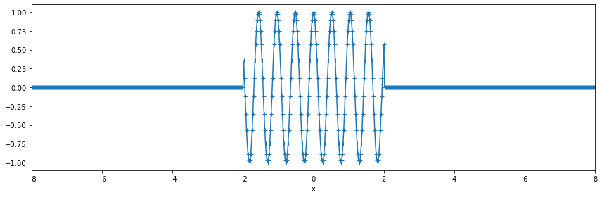
y = np.cos(2*np.pi*k0*x)
y[np.abs(x)>T/2]=0.
da = xr.DataArray(y, dims=('x',), coords={'x':x})
[22]:
fig, ax = plt.subplots(figsize=(12,4))
fig.set_tight_layout(True)
da.plot(ax=ax, marker='+', label='original signal')
ax.set_xlim([-8,8]);
Let’s take the Fourier transform
We will compare the Fourier transform with and without taking into consideration about the phase information.
[3]:
da_dft = xrft.dft(da, true_phase=True, true_amplitude=True) # Fourier Transform w/ consideration of phase
da_fft = xrft.fft(da)                                       # Fourier Transform w/ numpy.fft-like behavior
da_npft = npft.fft(da)
[4]:
k = da_dft.freq_x # wavenumber axis
TF_s = T/2*(np.sinc(T*(k-k0)) + np.sinc(T*(k+k0))) # Theoretical result of the Fourier transform
[26]:
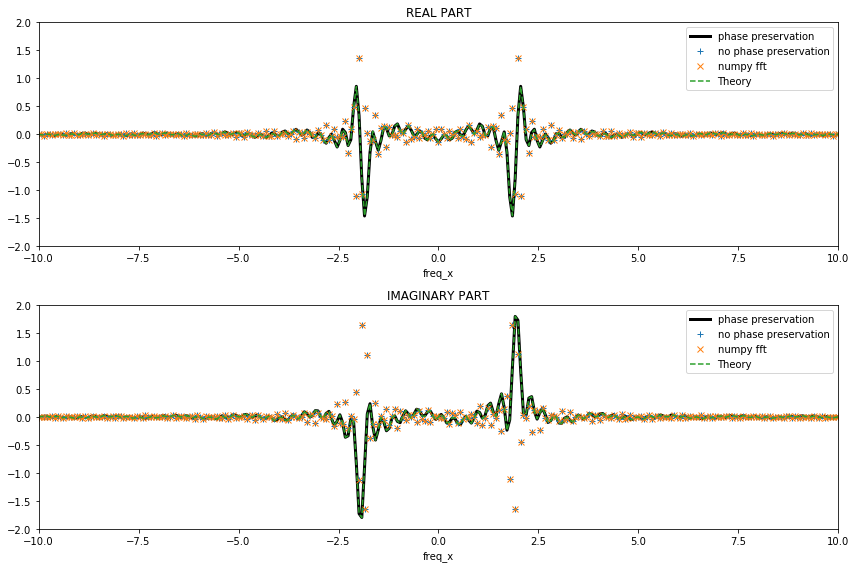
fig, (ax1,ax2) = plt.subplots(figsize=(12,8), nrows=2, ncols=1)
fig.set_tight_layout(True)

(da_dft.real).plot(ax=ax1, linestyle='-', lw=3, c='k', label='phase preservation')
((da_fft*dx).real).plot(ax=ax1, linestyle='', marker='+',label='no phase preservation')
ax1.plot(k, (npft.fftshift(da_npft)*dx).real, linestyle='', marker='x',label='numpy fft')
ax1.plot(k, TF_s.real, linestyle='--', label='Theory')
ax1.set_xlim([-10,10])
ax1.set_ylim([-2,2])
ax1.legend()
ax1.set_title('REAL PART')

(da_dft.imag).plot(ax=ax2, linestyle='-', lw=3, c='k', label='phase preservation')
((da_fft*dx).imag).plot(ax=ax2, linestyle='', marker='+', label='no phase preservation')
ax2.plot(k, (npft.fftshift(da_npft)*dx).imag, linestyle='', marker='x',label='numpy fft')
ax2.plot(k, TF_s.imag, linestyle='--', label='Theory')
ax2.set_xlim([-10,10])
ax2.set_ylim([-2,2])
ax2.legend()
ax2.set_title('IMAGINARY PART');
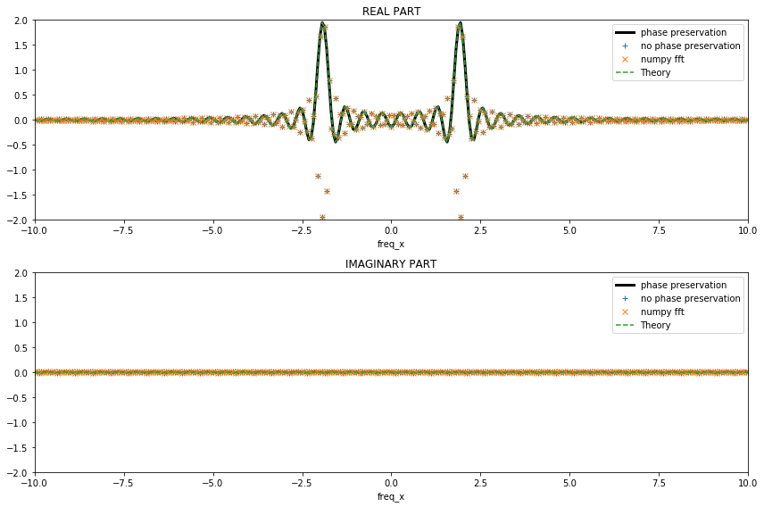
xrft.dft, xrft.fft (and npft.fft with careful npft.fftshifting) all give the same amplitudes as theory (as the coordinates of the original data was centered) but the latter two get the sign wrong due to losing the phase information. It is perhaps worth noting that the latter two (xrft.fft and npft.fft) require the amplitudes to be multiplied by \(dx\) to be consistent with theory while xrft.dft automatically takes care of this with the flag
true_amplitude=True:
Perform the inverse transform
[5]:
ida_dft = xrft.idft(da_dft, true_phase=True, true_amplitude=True) # Signal in direct space
ida_fft = xrft.ifft(da_fft)
[19]:
fig, ax = plt.subplots(figsize=(12,4))
fig.set_tight_layout(True)
ida_dft.real.plot(ax=ax, linestyle='-', c='k', lw=4, label='phase preservation')
ax.plot(x, ida_fft.real, linestyle='', marker='+', label='no phase preservation', alpha=.6) # w/out the phase information, the coordinates are lost
da.plot(ax=ax, ls='--', lw=3, label='original signal')
ax.plot(x, npft.ifft(da_npft).real, ls=':', label='inverse of numpy fft')
ax.set_xlim([-8,8])
ax.legend(loc='upper left');
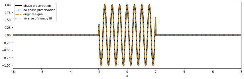
Although xrft.ifft misses the amplitude scaling (viz. resolution in wavenumber or frequency), since it is the inverse of the Fourier transform uncorrected for \(dx\), the result becomes consistent with xrft.idft. In other words, xrft.fft (and npft.fft) misses the \(dx\) scaling and xrft.ifft (and npft.ifft) misses the \(df\ (=1/(N\times dx))\) scaling. When applying the two operators in conjuction by doing ifft(fft()), there is a
\(1/N\ (=dx\times df)\) factor missing which is, in fact, arbitrarily included in the ``ifft` definition as a normalization factor <https://numpy.org/doc/stable/reference/routines.fft.html#module-numpy.fft>`__. By incorporating the right scalings in xrft.dft and xrft.idft, there is no more consideration of the number of data points (\(N\)):
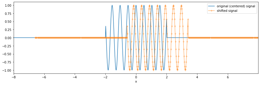
Synthetic data not centered around zero
Now let’s shift the coordinates so that they are not centered.
This is where the ``xrft`` magic happens. With the relevant flags, xrft’s dft can preserve information about the data’s location in its original space. This information is not preserved in a numpy fourier transform. This section demonstrates how to preserve this information using the true_phase=True, true_amplitude=True flags.
[26]:
nshift = 70                          # defining a shift
x0 = dx*nshift
nda = da.shift(x=nshift).dropna('x')
[27]:
fig, ax = plt.subplots(figsize=(12,4))
fig.set_tight_layout(True)
da.plot(ax=ax, label='original (centered) signal')
nda.plot(ax=ax, marker='+', label='shifted signal', alpha=.6)
ax.set_xlim([-8,nda.x.max()])
ax.legend();
We consider again the Fourier transform.
[28]:
nda_dft = xrft.dft(nda, true_phase=True, true_amplitude=True) # Fourier Transform w/ phase preservation
nda_fft = xrft.fft(nda)                                       # Fourier Transform w/out phase preservation
nda_npft = npft.fft(nda)
[29]:
nk = nda_dft.freq_x # wavenumber axis
TF_ns = T/2*(np.sinc(T*(nk-k0)) + np.sinc(T*(nk+k0)))*np.exp(-2j*np.pi*nk*x0) # Theoretical FT (Note the additional phase)
[30]:
fig, (ax1,ax2) = plt.subplots(figsize=(12,8), nrows=2, ncols=1)
fig.set_tight_layout(True)

(nda_dft.real).plot(ax=ax1, linestyle='-', lw=3, c='k', label='phase preservation')
((nda_fft*dx).real).plot(ax=ax1, linestyle='', marker='+',label='no phase preservation')
ax1.plot(nk, (npft.fftshift(nda_npft)*dx).real, linestyle='', marker='x',label='numpy fft')
ax1.plot(nk, TF_ns.real, linestyle='--', label='Theory')
ax1.set_xlim([-10,10])
ax1.set_ylim([-2.,2])
ax1.legend()
ax1.set_title('REAL PART')

(nda_dft.imag).plot(ax=ax2, linestyle='-', lw=3, c='k', label='phase preservation')
((nda_fft*dx).imag).plot(ax=ax2, linestyle='', marker='+', label='no phase preservation')
ax2.plot(nk, (npft.fftshift(nda_npft)*dx).imag, linestyle='', marker='x',label='numpy fft')
ax2.plot(nk, TF_ns.imag, linestyle='--', label='Theory')
ax2.set_xlim([-10,10])
ax2.set_ylim([-2.,2.])
ax2.legend()
ax2.set_title('IMAGINARY PART');
The expected additional phase (i.e. the complex term; \(e^{-i2\pi kx_0}\)) that appears in theory is retrieved with xrft.dft but not with xrft.fft nor npft.fft. This is because in npft.fft, the input data is expected to be centered around zero. In the current version of ``xrft``, the behavior of ``xrft.dft`` defaults to ``xrft.fft`` so set the flags ``true_phase=True`` and ``true_amplitude=True`` in order to have the results matching with theory.
Now, let’s take the inverse transform.
[31]:
inda_dft = xrft.idft(nda_dft, true_phase=True, true_amplitude=True) # Signal in direct space
inda_fft = xrft.ifft(nda_fft)
[39]:
fig, ax = plt.subplots(figsize=(12,4))
fig.set_tight_layout(True)
inda_dft.real.plot(ax=ax, linestyle='-', c='k', lw=4, label='phase preservation')
ax.plot(x[:len(inda_fft.real)], inda_fft.real, linestyle='', marker='o', alpha=.7,
        label='no phase preservation (w/out shifting)')
ax.plot(x[nshift:], inda_fft.real, linestyle='', marker='+', label='no phase preservation')
nda.plot(ax=ax, ls='--', lw=3, label='original signal')
ax.plot(x[nshift:], npft.ifft(nda_npft).real, ls=':', label='inverse of numpy fft')
ax.set_xlim([nda.x.min(),nda.x.max()])
ax.legend(loc='upper left');
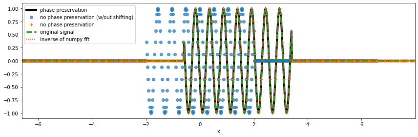
Note that we are only able to match the inverse transforms of xrft.ifft and npft.ifft to the data nda to it being Fourier transformed because we “know” the original data da was shifted by nshift datapoints as we see in x[nshift:] (compare the blue dots and orange crosses where without the knowledge of the shift, we may assume that the data were centered around zero). Using ``xrft.idft`` along with ``xrft.dft`` with the flags ``true_phase=True`` and
``true_amplitude=True`` automatically takes care of the information of shifted coordinates.
A case with real data
Load atmosheric temperature from the NMC reanalysis.
[4]:
da = xr.tutorial.open_dataset("air_temperature").air
da
[4]:
- time: 2920
- lat: 25
- lon: 53
- ...
[3869000 values with dtype=float32]
- lat(lat)float3275.0 72.5 70.0 ... 20.0 17.5 15.0
- standard_name :
- latitude
- long_name :
- Latitude
- units :
- degrees_north
- axis :
- Y
array([75. , 72.5, 70. , 67.5, 65. , 62.5, 60. , 57.5, 55. , 52.5, 50. , 47.5, 45. , 42.5, 40. , 37.5, 35. , 32.5, 30. , 27.5, 25. , 22.5, 20. , 17.5, 15. ], dtype=float32) - lon(lon)float32200.0 202.5 205.0 ... 327.5 330.0
- standard_name :
- longitude
- long_name :
- Longitude
- units :
- degrees_east
- axis :
- X
array([200. , 202.5, 205. , 207.5, 210. , 212.5, 215. , 217.5, 220. , 222.5, 225. , 227.5, 230. , 232.5, 235. , 237.5, 240. , 242.5, 245. , 247.5, 250. , 252.5, 255. , 257.5, 260. , 262.5, 265. , 267.5, 270. , 272.5, 275. , 277.5, 280. , 282.5, 285. , 287.5, 290. , 292.5, 295. , 297.5, 300. , 302.5, 305. , 307.5, 310. , 312.5, 315. , 317.5, 320. , 322.5, 325. , 327.5, 330. ], dtype=float32) - time(time)datetime64[ns]2013-01-01 ... 2014-12-31T18:00:00
- standard_name :
- time
- long_name :
- Time
array(['2013-01-01T00:00:00.000000000', '2013-01-01T06:00:00.000000000',
       '2013-01-01T12:00:00.000000000', ..., '2014-12-31T06:00:00.000000000',
       '2014-12-31T12:00:00.000000000', '2014-12-31T18:00:00.000000000'],
      dtype='datetime64[ns]')
- long_name :
- 4xDaily Air temperature at sigma level 995
- units :
- degK
- precision :
- 2
- GRIB_id :
- 11
- GRIB_name :
- TMP
- var_desc :
- Air temperature
- dataset :
- NMC Reanalysis
- level_desc :
- Surface
- statistic :
- Individual Obs
- parent_stat :
- Other
- actual_range :
- [185.16 322.1 ]
[6]:
Fda = xrft.dft(da.isel(time=0), dim="lat", true_phase=True, true_amplitude=True)
Fda
[6]:
- freq_lat: 25
- lon: 53
- (55.72721061044916-46.861821150779946j) ... (57.947560549433405+48.51852927393743j)
array([[ 55.72721061-46.86182115j, 54.88410513-45.81648436j, 54.44861105-45.4792758j , ..., 63.78368643-52.78354988j, 60.99712143-50.28091047j, 57.94756055-48.51852927j], [-38.90906614-66.9663849j , -38.90038095-67.92497252j, -38.544492 -68.17925905j, ..., -41.94737401-74.09175983j, -40.00936528-70.47655747j, -39.05651073-68.04032158j], [-77.82019891+12.50876021j, -79.02288653+10.06164636j, -80.34175059 +9.81548668j, ..., -86.83039434+26.4819109j , -84.02694401+23.31755583j, -81.26451369+21.4268003j ], ..., [-77.82019891-12.50876021j, -79.02288653-10.06164636j, -80.34175059 -9.81548668j, ..., -86.83039434-26.4819109j , -84.02694401-23.31755583j, -81.26451369-21.4268003j ], [-38.90906614+66.9663849j , -38.90038095+67.92497252j, -38.544492 +68.17925905j, ..., -41.94737401+74.09175983j, -40.00936528+70.47655747j, -39.05651073+68.04032158j], [ 55.72721061+46.86182115j, 54.88410513+45.81648436j, 54.44861105+45.4792758j , ..., 63.78368643+52.78354988j, 60.99712143+50.28091047j, 57.94756055+48.51852927j]]) - lon(lon)float32200.0 202.5 205.0 ... 327.5 330.0
- standard_name :
- longitude
- long_name :
- Longitude
- units :
- degrees_east
- axis :
- X
array([200. , 202.5, 205. , 207.5, 210. , 212.5, 215. , 217.5, 220. , 222.5, 225. , 227.5, 230. , 232.5, 235. , 237.5, 240. , 242.5, 245. , 247.5, 250. , 252.5, 255. , 257.5, 260. , 262.5, 265. , 267.5, 270. , 272.5, 275. , 277.5, 280. , 282.5, 285. , 287.5, 290. , 292.5, 295. , 297.5, 300. , 302.5, 305. , 307.5, 310. , 312.5, 315. , 317.5, 320. , 322.5, 325. , 327.5, 330. ], dtype=float32) - time()datetime64[ns]2013-01-01
- standard_name :
- time
- long_name :
- Time
array('2013-01-01T00:00:00.000000000', dtype='datetime64[ns]') - freq_lat(freq_lat)float64-0.192 -0.176 -0.16 ... 0.176 0.192
- spacing :
- 0.016000000000000014
array([-0.192, -0.176, -0.16 , -0.144, -0.128, -0.112, -0.096, -0.08 , -0.064,
       -0.048, -0.032, -0.016,  0.   ,  0.016,  0.032,  0.048,  0.064,  0.08 ,
        0.096,  0.112,  0.128,  0.144,  0.16 ,  0.176,  0.192])
The coordinate metadata is lost during the DFT (or any Fourier transform) operation so we need to specify the lag to retrieve the latitudes back in the inverse transform. The original latitudes are centered around 45\(^\circ\) so we set the lag to lag=45.
[8]:
Fda_1 = xrft.idft(Fda, dim="freq_lat", true_phase=True, true_amplitude=True, lag=45)
Fda_1
[8]:
- lat: 25
- lon: 53
- (296.2900085449223-7.014888176295515e-16j) ... (238.5999908447269+4.1703029862596966e-16j)
array([[296.29000854-7.01488818e-16j, 296.79000854-2.41028295e-15j, 297.1000061 -1.08051561e-15j, ..., 296.8999939 +2.07870428e-15j, 296.79000854+1.39068454e-15j, 296.6000061 +1.98243140e-15j], [295.8999939 -1.36617001e-16j, 296.19998169-3.08854147e-15j, 296.79000854-2.27797690e-16j, ..., 295.8999939 -2.06120304e-15j, 295.8999939 -7.63307736e-16j, 295.19998169+2.90958929e-15j], [296.6000061 +2.18513309e-15j, 296.19998169-5.34587573e-16j, 296.3999939 -1.70159409e-15j, ..., 295.3999939 -9.67078004e-16j, 295.1000061 -2.97325892e-15j, 294.69998169+2.84108954e-15j], ..., [250. +1.32015223e-15j, 249.79998779+5.34587573e-16j, 248.88999939-1.80369123e-15j, ..., 233.19999695+9.67078004e-16j, 236.38999939+3.00722368e-17j, 241.69999695+3.04528382e-15j], [243.79998779-1.32169378e-16j, 244.5 -4.76080394e-15j, 244.69999695-1.17678849e-15j, ..., 232.79998779+1.86297913e-15j, 235.29998779-3.02882224e-16j, 239.29998779-9.67078004e-16j], [241.19999695+5.26510200e-16j, 242.5 -1.34198513e-15j, 243.5 -3.83146461e-16j, ..., 232.79998779+2.46618241e-15j, 235.5 +3.62856196e-16j, 238.59999084+4.17030299e-16j]]) - lon(lon)float32200.0 202.5 205.0 ... 327.5 330.0
- standard_name :
- longitude
- long_name :
- Longitude
- units :
- degrees_east
- axis :
- X
array([200. , 202.5, 205. , 207.5, 210. , 212.5, 215. , 217.5, 220. , 222.5, 225. , 227.5, 230. , 232.5, 235. , 237.5, 240. , 242.5, 245. , 247.5, 250. , 252.5, 255. , 257.5, 260. , 262.5, 265. , 267.5, 270. , 272.5, 275. , 277.5, 280. , 282.5, 285. , 287.5, 290. , 292.5, 295. , 297.5, 300. , 302.5, 305. , 307.5, 310. , 312.5, 315. , 317.5, 320. , 322.5, 325. , 327.5, 330. ], dtype=float32) - time()datetime64[ns]2013-01-01
- standard_name :
- time
- long_name :
- Time
array('2013-01-01T00:00:00.000000000', dtype='datetime64[ns]') - lat(lat)float6415.0 17.5 20.0 ... 70.0 72.5 75.0
- spacing :
- 2.4999999999999964
array([15. , 17.5, 20. , 22.5, 25. , 27.5, 30. , 32.5, 35. , 37.5, 40. , 42.5,
       45. , 47.5, 50. , 52.5, 55. , 57.5, 60. , 62.5, 65. , 67.5, 70. , 72.5,
       75. ])
[20]:
fig, (ax1,ax2) = plt.subplots(figsize=(12,4), nrows=1, ncols=2)
da.isel(time=0).plot(ax=ax1)
Fda_1.real.plot(ax=ax2)
[20]:
<matplotlib.collections.QuadMesh at 0x1226607f0>
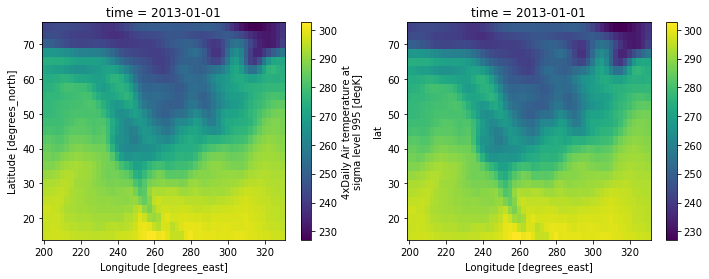
We see the inverse DFT of the Fourier transformed original temperature data returns the original data.
[ ]: