Example of Parseval’s theorem

import numpy as np
import numpy.testing as npt
import xarray as xr
import xrft
import numpy.fft as npft
import dask.array as dsar
import matplotlib.pyplot as plt
%matplotlib inline

First, we show that ``xrft.dft`` satisfies the Parseval’s theorem exactly for a non-windowed signal

For one-dimensional data:

\[\sum_x (da)^2 \Delta x = \sum_k \mathcal{F}(da)[\mathcal{F}(da)]^* \Delta k.\]

Generate synthetic data

Nx = 40
dx = np.random.rand()
da = xr.DataArray(
        np.random.rand(Nx) + 1j * np.random.rand(Nx),
        dims="x",
        coords={"x": dx * (np.arange(-Nx // 2, -Nx // 2 + Nx)
                           + np.random.randint(-Nx // 2, Nx // 2)
                          )
               },
                 )

###############
# Assert Parseval's using xrft.dft
###############
FT = xrft.dft(da, dim="x", true_phase=True, true_amplitude=True)
npt.assert_almost_equal(
        (np.abs(da) ** 2).sum() * dx, (np.abs(FT) ** 2).sum() * FT["freq_x"].spacing
                       )

###############
# Assert Parseval's using xrft.power_spectrum with scaling='density'
###############
ps = xrft.power_spectrum(da, dim="x")
npt.assert_almost_equal(
        ps.sum(),
        (np.abs(da) ** 2).sum() * dx
                       )

For two-dimensional data:

\[\sum_x \sum_y (da)^2 \Delta x \Delta y = \sum_k \sum_l \mathcal{F}(da)\mathcal{F}(da)^* \Delta k \Delta l.\]

Generate synthetic data

Ny = 60
dx, dy = (np.random.rand(), np.random.rand())
da2 = xr.DataArray(
        np.random.rand(Nx, Ny) + 1j * np.random.rand(Nx, Ny),
        dims=["x", "y"],
        coords={"x": dx
                * (
                    np.arange(-Nx // 2, -Nx // 2 + Nx)
                    + np.random.randint(-Nx // 2, Nx // 2)
                ),
                "y": dy
                * (
                    np.arange(-Ny // 2, -Ny // 2 + Ny)
                    + np.random.randint(-Ny // 2, Ny // 2)
                ),
              },
                  )

###############
# Assert Parseval's using xrft.dft
###############
FT2 = xrft.dft(da2, dim=["x", "y"], true_phase=True, true_amplitude=True)
npt.assert_almost_equal(
        (np.abs(FT2) ** 2).sum() * FT2["freq_x"].spacing * FT2["freq_y"].spacing,
        (np.abs(da2) ** 2).sum() * dx * dy,
                       )

###############
# Assert Parseval's using xrft.power_spectrum with scaling='density'
###############
ps2 = xrft.power_spectrum(da2, dim=["x", "y"])
npt.assert_almost_equal(
        ps2.sum(),
        (np.abs(da2) ** 2).sum() * dx * dy
                       )

###############
# Assert Parseval's using xrft.power_spectrum with scaling='spectrum'
###############
ps2 = xrft.power_spectrum(da2, dim=["x", "y"], scaling='spectrum')
npt.assert_almost_equal(
        ps2.sum() / (ps2.freq_x.spacing * ps2.freq_y.spacing),
        (np.abs(da2) ** 2).sum() * dx * dy,
                       )

Now, we show how Parseval’s theorem is approximately satisfied for windowed data

\[\frac{1}{\langle w^2\rangle} \sum_x (w\ da)^2 \Delta x = \sum_x (da)^2 \Delta x \approx \frac{1}{\langle w^2\rangle} \sum_k \mathcal{F}(w)\circ\mathcal{F}(da)[\mathcal{F}(w)\circ\mathcal{F}(da)]^* \Delta k,\]

where \(w\) is the windowing function, \(\circ\) is the convolution operator and \(\langle \cdot \rangle\) is the area sum, namely, \(\sum_x\).

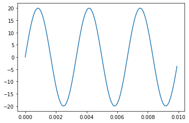
Generate synthetic data: A \(300\)Hz sine wave with an RMS\(^2\) of \(200\).

A = 20
fs = 1e4
n_segments = int(fs // 10)
fsig = 300
ii = int(fsig * n_segments // fs)  # frequency index of fsig

tt = np.arange(fs) / fs
x = A * np.sin(2 * np.pi * fsig * tt)
plt.plot(tt[:100],x[:100]);

Assert Parseval’s for different windowing functions

Depending on the scaling flag, a different correction is applied to the windowed spectrum:

• scaling='density': Energy correction - this corrects for the energy (integral) of the spectrum. It is typically applied to the power spectral density (including cross power spectral density) and rescales the spectrum by 1.0 / (window**2).mean(). It ensures that the integral of the spectral density (approximately) matches the RMS\(^2\) of the signal (i.e. that Parseval’s theorem is satisfied).

• scaling='spectrum': Amplitude correction - this corrects the amplitude of peaks in the spectrum and rescales the spectrum by 1.0 / window.mean()**2. It is typically applied to the power spectrum (i.e. not density) and is most useful in strongly periodic signals. It ensures, for example, that the peak in the power spectrum of a 300 Hz sine wave with RMS\(^2 = 200\) has a magnitude of \(200\).

These scalings replicate the default behaviour of scipy spectral functions like scipy.signal.periodogram and scipy.signal.welch (cf. Section 11.5.2. of Bendat & Piersol, 2011; Section 10.3 of Brandt, 2011).

RMS = np.sqrt(np.mean((x**2)))

windows = np.array([["hann","bartlett"],["tukey","flattop"]])

Check the energy correction for ``scaling=’density’``: With window_correction=True, the spectrum integrates to RMS\(^2\).

fig, axes = plt.subplots(figsize=(13,10), nrows=2, ncols=2)
fig.set_tight_layout(True)

for window_type in windows.ravel():

    x_da = xr.DataArray(x, coords=[tt], dims=["x"]).chunk({"x": n_segments})

    ps = xrft.power_spectrum(
        x_da,
        dim="x",
        window=window_type,
        chunks_to_segments=True,
        window_correction=True,
    ).mean("x_segment")

    ps.plot(ax=axes[np.where(windows==window_type)[0][0],np.where(windows==window_type)[1][0]])
    axes[np.where(windows==window_type)[0][0],np.where(windows==window_type)[1][0]].set_title(window_type, fontsize=15)

    npt.assert_allclose(
        np.trapz(ps.values, ps.freq_x.values),
        RMS**2,
        rtol=1e-3
    )

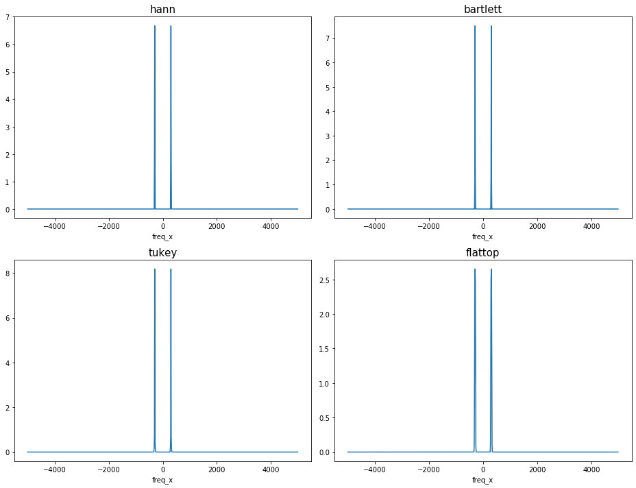
The maximum amplitude differs amongst cases with different windows due to the difference in noise floor.

Check the amplitude correction for ``scaling=’spectrum’``: With window_correction=True, the peak of the two-sided spectrum has a magnitude of RMS\(^2/2\).

fig, axes = plt.subplots(figsize=(13,10), nrows=2, ncols=2)
fig.set_tight_layout(True)

for window_type in windows.ravel():

    x_da = xr.DataArray(x, coords=[tt], dims=["x"]).chunk({"x": n_segments})

    ps = xrft.power_spectrum(
        x_da,
        dim="x",
        window=window_type,
        chunks_to_segments=True,
        scaling="spectrum",
        window_correction=True,
    ).mean("x_segment")

    ps.plot(ax=axes[np.where(windows==window_type)[0][0],np.where(windows==window_type)[1][0]])
    axes[np.where(windows==window_type)[0][0],np.where(windows==window_type)[1][0]].set_title(window_type, fontsize=15)

    # The factor of 0.5 is there because we're checking the two-sided spectrum
    npt.assert_allclose(ps.sel(freq_x=fsig), 0.5 * RMS**2)

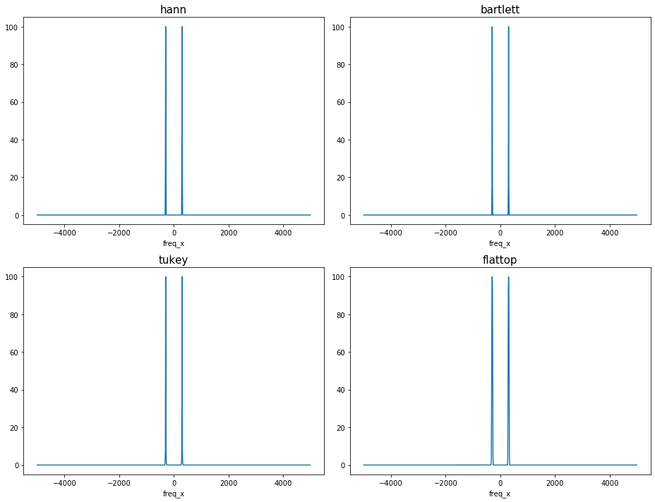
The maximum amplitudes are now all the same amongst different windows applied with the amplitude correction.