[1]:
import numpy as np
import numpy.testing as npt
import xarray as xr
import xrft
import dask.array as dsar
from matplotlib import colors
import matplotlib.pyplot as plt
%matplotlib inline
Parallelized Bartlett’s Method
For long data sets that have reached statistical equilibrium, it is useful to chunk the data, calculate the periodogram for each chunk and then take the average to reduce variance.
[2]:
n = int(2**8)
da = xr.DataArray(np.random.rand(n,int(n/2),int(n/2)), dims=['time','y','x'])
da
[2]:
<xarray.DataArray (time: 256, y: 128, x: 128)>
array([[[ 0.493341,  0.28303 , ...,  0.434256,  0.616031],
        [ 0.777314,  0.629644, ...,  0.152931,  0.445424],
        ...,
        [ 0.562456,  0.022227, ...,  0.88538 ,  0.054687],
        [ 0.381456,  0.908454, ...,  0.843443,  0.706326]],

       [[ 0.469143,  0.241104, ...,  0.249369,  0.830898],
        [ 0.283305,  0.438634, ...,  0.893666,  0.242556],
        ...,
        [ 0.897823,  0.187038, ...,  0.977466,  0.270899],
        [ 0.252733,  0.425873, ...,  0.228847,  0.954393]],

       ...,
       [[ 0.936424,  0.793693, ...,  0.406293,  0.272336],
        [ 0.917752,  0.83908 , ...,  0.954489,  0.151129],
        ...,
        [ 0.081756,  0.016332, ...,  0.524886,  0.87095 ],
        [ 0.677224,  0.41488 , ...,  0.12199 ,  0.689685]],

       [[ 0.193302,  0.113419, ...,  0.083486,  0.784332],
        [ 0.695728,  0.376776, ...,  0.278004,  0.026373],
        ...,
        [ 0.677775,  0.255296, ...,  0.112851,  0.46325 ],
        [ 0.598086,  0.529324, ...,  0.267431,  0.65419 ]]])
Dimensions without coordinates: time, y, x
One dimension
Discrete Fourier Transform
[3]:
daft = xrft.dft(da.chunk({'time':int(n/4)}), dim=['time'], shift=False , chunks_to_segments=True).compute()
daft
[3]:
<xarray.DataArray 'fftn-917988d0ce7d7da01b5f7a3cf2bb9a26' (time_segment: 4, freq_time: 64, y: 128, x: 128)>
array([[[[ 30.737014+0.j      , ...,  31.659135+0.j      ],
         ...,
         [ 31.308938+0.j      , ...,  31.768846+0.j      ]],

        ...,
        [[  1.928097-0.118076j, ...,   0.732440+2.07656j ],
         ...,
         [  0.225814+1.256083j, ...,   0.244113-1.276807j]]],


       ...,
       [[[ 37.777908+0.j      , ...,  30.996848+0.j      ],
         ...,
         [ 28.650088+0.j      , ...,  35.362874+0.j      ]],

        ...,
        [[ -1.780642+0.477772j, ...,   2.575858+1.71943j ],
         ...,
         [  3.149759-2.664934j, ...,   1.872009-2.977565j]]]])
Coordinates:
  * time_segment       (time_segment) int64 0 1 2 3
  * freq_time          (freq_time) float64 0.0 0.01562 0.03125 0.04688 ...
  * y                  (y) int64 0 1 2 3 4 5 6 7 8 9 10 11 12 13 14 15 16 17 ...
  * x                  (x) int64 0 1 2 3 4 5 6 7 8 9 10 11 12 13 14 15 16 17 ...
    freq_time_spacing  float64 0.01562
[4]:
data = da.chunk({'time':int(n/4)}).data
data_rs = data.reshape((4,int(n/4),int(n/2),int(n/2)))
da_rs = xr.DataArray(data_rs, dims=['time_segment','time','y','x'])
da1 = xr.DataArray(dsar.fft.fftn(data_rs, axes=[1]).compute(),
                   dims=['time_segment','freq_time','y','x'])
da1
[4]:
<xarray.DataArray (time_segment: 4, freq_time: 64, y: 128, x: 128)>
array([[[[ 30.737014+0.j      , ...,  31.659135+0.j      ],
         ...,
         [ 31.308938+0.j      , ...,  31.768846+0.j      ]],

        ...,
        [[  1.928097-0.118076j, ...,   0.732440+2.07656j ],
         ...,
         [  0.225814+1.256083j, ...,   0.244113-1.276807j]]],


       ...,
       [[[ 37.777908+0.j      , ...,  30.996848+0.j      ],
         ...,
         [ 28.650088+0.j      , ...,  35.362874+0.j      ]],

        ...,
        [[ -1.780642+0.477772j, ...,   2.575858+1.71943j ],
         ...,
         [  3.149759-2.664934j, ...,   1.872009-2.977565j]]]])
Dimensions without coordinates: time_segment, freq_time, y, x
We assert that our calculations give equal results.
[5]:
npt.assert_almost_equal(da1, daft.values)
Power Spectrum
[6]:
ps = xrft.power_spectrum(da.chunk({'time':int(n/4)}), dim=['time'], chunks_to_segments=True)
ps
[6]:
<xarray.DataArray 'concatenate-183433100cd82e429170a4fe2f9c4cbb' (time_segment: 4, freq_time: 64, y: 128, x: 128)>
dask.array<truediv, shape=(4, 64, 128, 128), dtype=float64, chunksize=(1, 32, 128, 128)>
Coordinates:
  * time_segment       (time_segment) int64 0 1 2 3
  * freq_time          (freq_time) float64 -0.5 -0.4844 -0.4688 -0.4531 ...
  * y                  (y) int64 0 1 2 3 4 5 6 7 8 9 10 11 12 13 14 15 16 17 ...
  * x                  (x) int64 0 1 2 3 4 5 6 7 8 9 10 11 12 13 14 15 16 17 ...
    freq_time_spacing  float64 0.01562
Taking the mean over the segments gives the Barlett’s estimate.
[7]:
ps = ps.mean(['time_segment','y','x'])
ps
[7]:
<xarray.DataArray 'concatenate-183433100cd82e429170a4fe2f9c4cbb' (freq_time: 64)>
dask.array<mean_agg-aggregate, shape=(64,), dtype=float64, chunksize=(32,)>
Coordinates:
  * freq_time          (freq_time) float64 -0.5 -0.4844 -0.4688 -0.4531 ...
    freq_time_spacing  float64 0.01562
[8]:
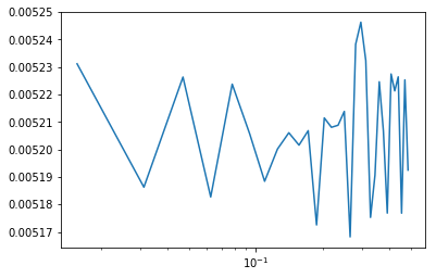
fig, ax = plt.subplots()
ax.semilogx(ps.freq_time[int(n/8)+1:], ps[int(n/8)+1:])
[8]:
[<matplotlib.lines.Line2D at 0x10ebc9518>]
Two dimension
Discrete Fourier Transform
[9]:
daft = xrft.dft(da.chunk({'y':32,'x':32}), dim=['y','x'], shift=False , chunks_to_segments=True).compute()
daft
[9]:
<xarray.DataArray 'fftn-8077935acd6b48b40d6593c688c326b2' (time: 256, y_segment: 4, freq_y: 32, x_segment: 4, freq_x: 32)>
array([[[[[ 505.090962 +0.j      , ...,    3.673241 +2.033024j],
          ...,
          [ 506.979486 +0.j      , ...,    2.672219 +8.645102j]],

         ...,
         [[  -1.746757 -1.347122j, ...,   -2.183099+17.472835j],
          ...,
          [   3.450049 +3.832201j, ...,   -4.072164 -7.279733j]]],


        ...,
        [[[ 504.971751 +0.j      , ...,   -6.610465-12.385931j],
          ...,
          [ 512.756185 +0.j      , ...,   -4.344255 -8.458134j]],

         ...,
         [[  -7.979198 -7.454325j, ...,   -2.962019 +6.43059j ],
          ...,
          [   4.024805 +3.72519j , ...,   -8.242673 -8.259182j]]]],


       ...,
       [[[[ 518.573138 +0.j      , ...,    0.573928-10.006888j],
          ...,
          [ 520.423164 +0.j      , ...,   -1.110088 +0.141936j]],

         ...,
         [[   2.043005 -3.116515j, ...,    8.697924 -5.116488j],
          ...,
          [   3.702009 -7.202762j, ...,  -12.007770 +3.514272j]]],


        ...,
        [[[ 523.615806 +0.j      , ...,   -9.301065 +4.935474j],
          ...,
          [ 521.535950 +0.j      , ...,    6.826755 +1.688166j]],

         ...,
         [[   2.157400-14.676636j, ...,   -1.865237-11.408717j],
          ...,
          [   0.651302 +0.531716j, ...,    5.861882 +5.968681j]]]]])
Coordinates:
  * time            (time) int64 0 1 2 3 4 5 6 7 8 9 10 11 12 13 14 15 16 17 ...
  * y_segment       (y_segment) int64 0 1 2 3
  * freq_y          (freq_y) float64 0.0 0.03125 0.0625 0.09375 0.125 0.1562 ...
  * x_segment       (x_segment) int64 0 1 2 3
  * freq_x          (freq_x) float64 0.0 0.03125 0.0625 0.09375 0.125 0.1562 ...
    freq_y_spacing  float64 0.03125
    freq_x_spacing  float64 0.03125
[10]:
data = da.chunk({'y':32,'x':32}).data
data_rs = data.reshape((256,4,32,4,32))
da_rs = xr.DataArray(data_rs, dims=['time','y_segment','y','x_segment','x'])
da2 = xr.DataArray(dsar.fft.fftn(data_rs, axes=[2,4]).compute(),
                   dims=['time','y_segment','freq_y','x_segment','freq_x'])
da2
[10]:
<xarray.DataArray (time: 256, y_segment: 4, freq_y: 32, x_segment: 4, freq_x: 32)>
array([[[[[ 505.090962 +0.j      , ...,    3.673241 +2.033024j],
          ...,
          [ 506.979486 +0.j      , ...,    2.672219 +8.645102j]],

         ...,
         [[  -1.746757 -1.347122j, ...,   -2.183099+17.472835j],
          ...,
          [   3.450049 +3.832201j, ...,   -4.072164 -7.279733j]]],


        ...,
        [[[ 504.971751 +0.j      , ...,   -6.610465-12.385931j],
          ...,
          [ 512.756185 +0.j      , ...,   -4.344255 -8.458134j]],

         ...,
         [[  -7.979198 -7.454325j, ...,   -2.962019 +6.43059j ],
          ...,
          [   4.024805 +3.72519j , ...,   -8.242673 -8.259182j]]]],


       ...,
       [[[[ 518.573138 +0.j      , ...,    0.573928-10.006888j],
          ...,
          [ 520.423164 +0.j      , ...,   -1.110088 +0.141936j]],

         ...,
         [[   2.043005 -3.116515j, ...,    8.697924 -5.116488j],
          ...,
          [   3.702009 -7.202762j, ...,  -12.007770 +3.514272j]]],


        ...,
        [[[ 523.615806 +0.j      , ...,   -9.301065 +4.935474j],
          ...,
          [ 521.535950 +0.j      , ...,    6.826755 +1.688166j]],

         ...,
         [[   2.157400-14.676636j, ...,   -1.865237-11.408717j],
          ...,
          [   0.651302 +0.531716j, ...,    5.861882 +5.968681j]]]]])
Dimensions without coordinates: time, y_segment, freq_y, x_segment, freq_x
We assert that our calculations give equal results.
[11]:
npt.assert_almost_equal(da2, daft.values)
Power Spectrum
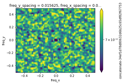
[14]:
ps = xrft.power_spectrum(da.chunk({'time':1,'y':64,'x':64}), dim=['y','x'],
                         chunks_to_segments=True, window='True', detrend='linear')
ps = ps.mean(['time','y_segment','x_segment'])
ps
[14]:
<xarray.DataArray 'concatenate-34ef1d78d80632d6b25c65df82f67753' (freq_y: 64, freq_x: 64)>
dask.array<mean_agg-aggregate, shape=(64, 64), dtype=float64, chunksize=(32, 32)>
Coordinates:
  * freq_y          (freq_y) float64 -0.5 -0.4844 -0.4688 -0.4531 -0.4375 ...
  * freq_x          (freq_x) float64 -0.5 -0.4844 -0.4688 -0.4531 -0.4375 ...
    freq_y_spacing  float64 0.01562
    freq_x_spacing  float64 0.01562
[19]:
fig, ax = plt.subplots()
ps.plot(ax=ax, norm=colors.LogNorm(), vmin=6.5e-4, vmax=7.5e-4)
[19]:
<matplotlib.collections.QuadMesh at 0x1210117b8>
[ ]: